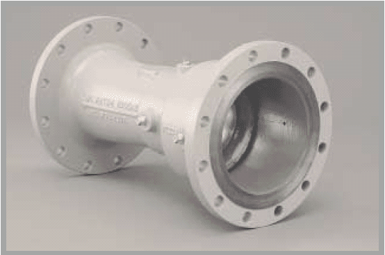
Pressure Vessel, Nonimpact Design
Based on the classical Venturi design, nonimpact Venturi meters are those that sense only axial components of the line fluid’s velocity profile; nonaxial vectors are considered insignificant in normalized piping. The resulting flow meter has a discharge coefficient (CD) that approaches a value of one, is not a function of fluid velocity and beta ratio (d/D), and is constant above a given threshold pipe Reynolds number. In general, designs that utilize this flow metering mechanism are less sensitive to upstream pipe fittings than those designs that employ other types of pressure sensation.
The BVT nonimpact design conforms to all those characteristics that make Venturi meters the preferred flow meter when accuracy, reliability, and low permanent pressure loss are required. The value and performance of the nonimpact BVT CD indicates an extremely efficient metering shape and independence of line velocity; only pipe Reynolds number (RD) is a concern. If the pipe Reynolds number is greater than 75 000, the substantiated uncertainty of the BVT design is better than ± 0.50%; for RD < 75 000, CD is known and repeatable.
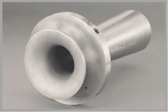
Insert-Type, Impact Design
Unlike the nonimpact design, insert-type, impact Venturi meters do sense a nonaxial velocity component in their high-pressure sensation. As a result, the meter discharge coefficient is dependent on beta ratio; however, CD is not a function of line velocity and is still constant above a given threshold pipe Reynolds number.
The BVT impact flow meter is a cost-effective alternative to the nonimpact pressure vessel design. While slightly more sensitive to upstream piping than the nonimpact design, these insert-type Venturi meters provide the same accuracy, reliability, and low pressure loss as that of the nonimpact design.
Though a function of beta ratio, the impact BVT CD provides the same efficient metering shape and independence from line velocity as the nonimpact BVT: If RD ≥ 75 000, then the uncertainty is better than
± 0.50%; for RD < 75 000, CD is predictable and repeatable. Contact Wyatt Engineering for further information.
Installation Effects
The differential pressure produced by the BVT design is an indication of the difference in the kinetic energy of the line fluid between the high- and low- pressure taps. Due to differing velocity profiles, a given flow rate can possess different kinetic energies, and thereby introduce errors in the indicated flow rate. This is the essence of the study of installation effects and allows for the calculation of installed uncertainty.
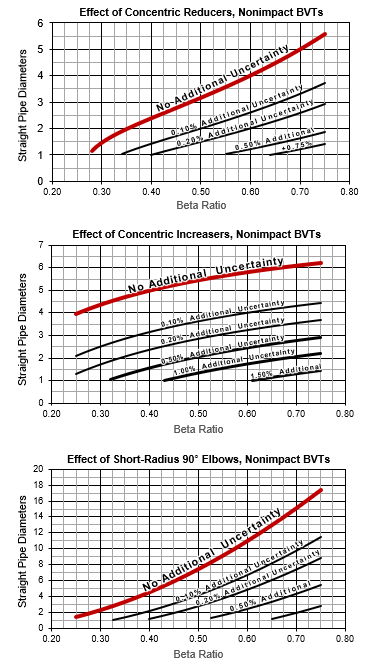
These curves to the right summarize the results of flow tests on nonimpact BVT flow meters. The “nonimpact” term reflects the condition that neither the high- nor the low-pressure tap senses nonaxial velocity components (sometimes imprecisely labeled “static tap”) The most common Wyatt Engineering models appropriate for these data are: BVT-B, BVT-CI, BVT-F, and BVT -U.
The test results show a clear relationship between the installation error function, EI , and β, the diameter ratio:
EI=0 .
In other words, meter sensitivity to an upstream disturbance decreases with decreasing diameter ratio (d/D), or the smaller the beta, the smaller the effect of upstream piping. Note that a similar relationship exists for orifice meters, flow nozzles, and nozzle Venturi meters. Simple enough, but here’s the rub:
∆H=∞ ,
the smaller the beta ratio, the higher the permanent pressure loss, ΔH. While the desire is to minimize both the specific headloss and installed uncertainty, sometimes increased permanent pressure loss is the price paid for improving the installed accuracy.
Flow patterns that change the behavior of the discharge coefficient can be caused by pipe fittings, Reynolds number, and/or pipe surface/diameter irregularities. From flow testing, we have learned that nonrotational, irregular flow patterns, that is, those caused by reducers, single elbows, etc., are self-attenuating, while irregular flow patterns that are rotational, for example, those caused by two elbows direct-coupled in perpendicular planes, are relatively stable and users should consider flow straighteners in such cases.
To determine the installed uncertainty, add the installation effect to the BVT uncertainty. The standard uncertainty is ±0.50% for Wyatt’s QS9001 calibrated meters, and (generally) ±0.25% for independently flow calibrated meters. These uncertainties are stated at a 95% confidence interval and should not be applied to other meter designs or models.
With respect to downstream piping requirements, pipe fittings, valves, etc. may be direct-coupled to the outlet of the BVT Venturi meter without affecting the accuracy. Note that some meters’ recovery sections are truncated, so direct-coupling a butterfly valve may, in some instances, cause the valve disk to interfere with the meter outlet and full valve disk movement may not be possible. Let us know if this configuration is required and the meter outlet will be modified accordingly. It should be noted also that the pressure loss of the direct- or close-coupled valve or pipe fitting will be somewhat higher than is calculated assuming a blunt velocity profile. If this is a concern, please contact Wyatt Engineering for further assistance.
Installation Effects (cont.)
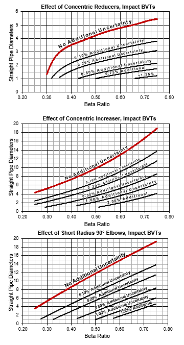
The curves shown above summarize the results of flow tests on impact BVT flow meters. In this case, the term “impact” indicates the high-pressure tap senses velocity components, both axial and nonaxial. This is due to the location of the high-pressure tap located either behind the meter inlet cone or at the intersection of the converging section and the upstream pipe. Meters employing this type of high-pressure sensation are sometimes – though incorrectly – referred to as using “full or partial Pitot effects.” Due to the nonaxial velocity component that influences the high-pressure sensation, the meter discharge coefficient (CD) is dependent on beta ratio, independent of line velocity, and still constant for pipe Reynolds numbers greater than about
75 000. The impact design typically refers to insert-type meters. The most common Wyatt Engineering models appropriate for the use of these data are: BVT-IF, BVT-IL, and BVT-IP.
Energy Considerations
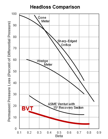
Energy loss, called specific headloss, is typically expressed in terms of pounds per square inch, inches of water column, kilopascals, etc. Losses for some different meter types are shown in Figure 1. In terms of generalized units, however, the true description is “Units of Energy per Units of Mass Flow.”
Consequently, the specific headloss of a meter, fitting, etc., represents an ongoing energy expense, “the cost of doing business,” and it is everyone’s duty to minimize that cost. For reference, a BVT sized for the same differential pressure consumes is less than one-eighth the energy of an orifice plate.
Pressure measured at a given point that does not have a nonaxial velocity vector is an indirect indication of the potential energy content of the flowing fluid at that cross section. Consequently, pressure drop is a measure of the energy dissipated between two points.
Uncertainty Substantiation
Uncertainty without Flow Calibration
The vast majority of BVT flow meters are provided without flow calibration. This is due to our ability to substantiate the uncertainty of the BVT to within ± 0.50% of indicated flow rate for pipe Reynolds numbers greater than 75 000.
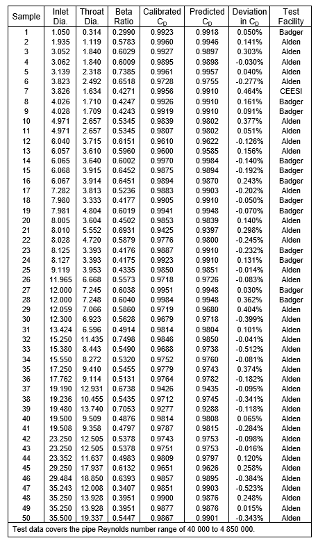
For the BVT meter design, there is a “true” discharge coefficient (CD). The true CD can be estimated only through repeated observations, but those observations (flow calibrations) will have uncertainties associated with them. The observed CD, therefore, equals the true CD plus the observed uncertainty band. The error on the estimated discharge coefficient, CD, approaches zero as the number of flow calibrations approaches infinity.
Since there are not an infinite number of flow calibrations, we must consider the contribution of the finite sample size to the combined uncertainty. Note that this allowance, formerly referred to as precision, is often neglected in many uncertainty calculations provided by the ill-informed or inexperienced. It is necessary, it cannot be ignored because it accounts for the finite size of the sample.
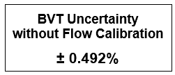
For the calibrations shown, the standard uncertainty of the data is ± 0.241% and consideration for the small sample is ± 0.069%. Together, this provides a combined uncertainty of ± 0.251%, which, in turn, results in an expanded uncertainty of ± 0.492% at a 95% confidence interval.
The method outlined above is the correct approach; anything else is sales talk.
Uncertainty is a calculated value, not an opinion.